Forests of temperate Europe in the light of open data, open source software and SQL

According to the interpretation manual of the EU habitat directive some forests of community interest in the region of the temperate Europe are:

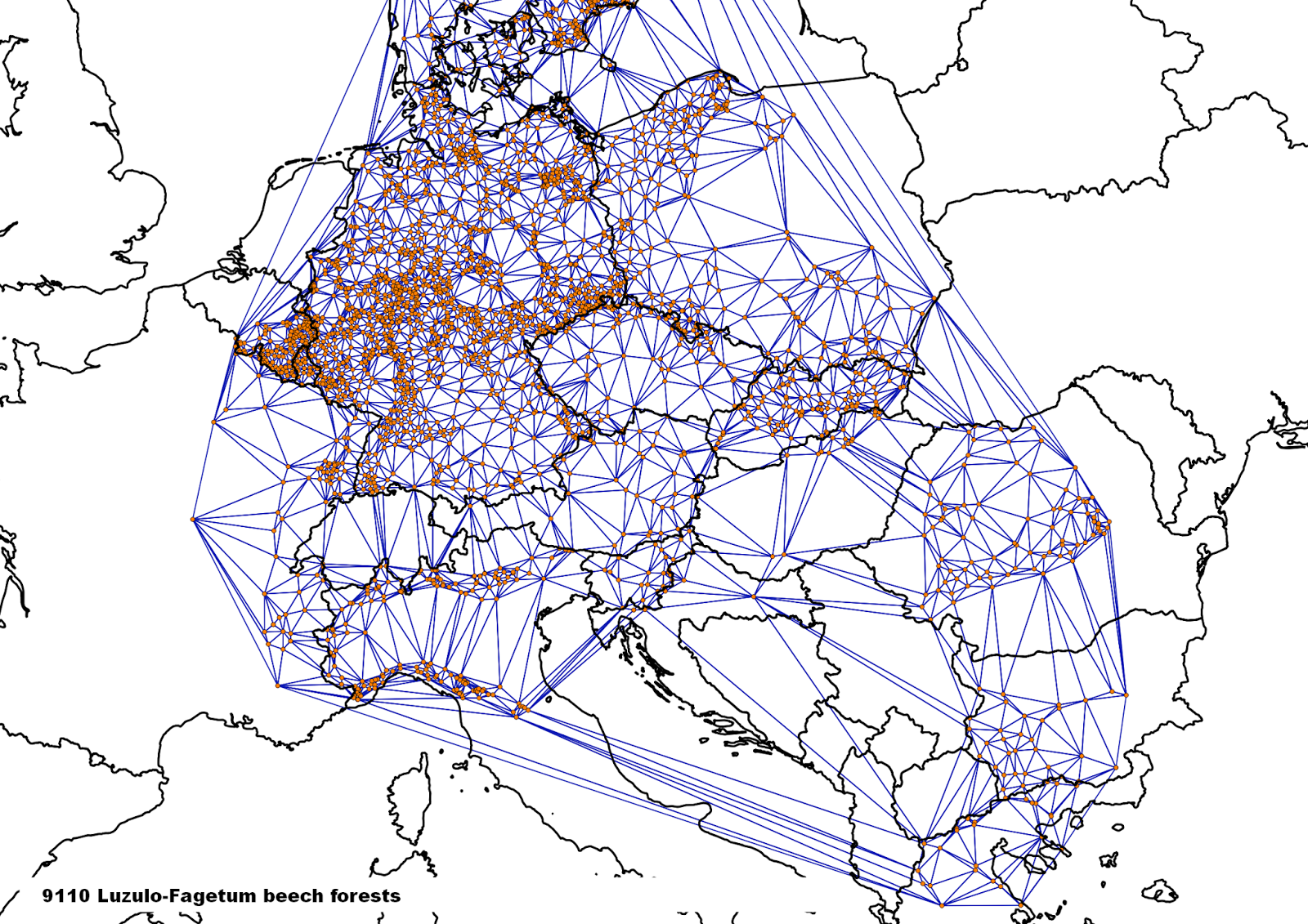
• 9110 Luzulo-Fagetum beech forests 
• 9120 Atlantic acidophilous beech forests with Ilex and sometimes also Taxus in the shrublayer (Quercinion robori-petraeae or Ilici-Fagenion)
• 9130 Asperulo-Fagetum beech forests
• 9140 Medio-European subalpine beech woods with Acer and Rumex arifolius
• 9150 Medio-European limestone beech forests of the Cephalanthero-Fagion
• 9160 Sub-Atlantic and medio-European oak or oakhornbeam forests of the Carpinion betuli
• 9170 Galio-Carpinetum oak-hornbeam forests
• 9180 * Tilio-Acerion forests of slopes, screes and ravines
• 9190 Old acidophilous oak woods with Quercus robur on sandy plains

Some open ingredients for baking an analysis around these forests:

• Natura 2000 data - the European network of protected sites
• Natural Earth Admin 0 – Countries
• SQLite - an open software library that implements a self-contained, serverless, zero-configuration, transactional SQL database engine
• SpatiaLite - open source library to extend the SQLite core to support fully fledged Spatial SQL capabilities
• GDAL/OGR
• QGIS

First download the spatialite version of the Natura 2000 data and have a quick look into the database by ogrinfo:

ogrinfo Natura2000_end2014.sqlite
INFO: Open of `Natura2000_end2014.sqlite'
      using driver `SQLite' successful.
1: natura2000polygon (Multi Polygon)

Beside the spatial data of protected areas within the Natura 2000 network (multipolygon layer: natura2000polygon), the database version of this data inlcudes also already additional informations connected to the protected areas (bioregion, contacts, designation status, directive species, habitat classes, habitats, impact, management, meta data, natura 2000 sites, other species, species).

Let's have a deeper look into the spatialite database (simplified by e.g. the spatialite-gui) and do some non-spatial SQL queries; e.g. filtering/querying the data and creating a view of protected areas including 9110 Luzulo-Fagetum beech forests:

# create view with protected areas including 9110 Luzulo-Fagetum beech forests based on the non-spatial table HABITATS
CREATE VIEW "vhabitat9110" AS
SELECT "SITECODE" AS "SITECODE", "HABITATCODE" AS "HABITATCODE",
    "COVER_HA" AS "COVER_HA", "REPRESENTATIVITY" AS "REPRESENTATIVITY",
    "RELSURFACE" AS "RELSURFACE", "CONSERVATION" AS "CONSERVATION",
    "GLOBAL_ASSESMENT" AS "GLOBAL_ASSESMENT", "DATAQUALITY" AS "DATAQUALITY",
    "PERCENTAGE_COVER" AS "PERCENTAGE_COVER"
FROM "HABITATS"
WHERE "HABITATCODE" = 9110
ORDER BY "SITECODE";

A view is some kind of a filtered/queried view of data organized like a table.

Just do it analogously for the other forest habitat types.

Then implement a spatial view of the data for later loading it to GIS:

# join the view created in the step before (vhabitat9110) with the spatial layer (Natura2000polygon) of the spatialite database.
CREATE VIEW "svhabitat9110" AS
SELECT "a"."ROWID" AS "ROWID", "a"."PK_UID" AS "PK_UID",
    "a"."SITECODE" AS "SITECODE", "a"."SITENAME" AS "SITENAME",
    "a"."RELEASE_DA" AS "RELEASE_DA", "a"."MS" AS "MS",
    "a"."SITETYPE" AS "SITETYPE", "a"."Geometry" AS "Geometry",
    "b"."SITECODE" AS "SITECODE_1", "b"."HABITATCODE" AS "HABITATCODE",
    "b"."COVER_HA" AS "COVER_HA", "b"."REPRESENTATIVITY" AS "REPRESENTATIVITY",
    "b"."RELSURFACE" AS "RELSURFACE", "b"."CONSERVATION" AS "CONSERVATION",
    "b"."GLOBAL_ASSESMENT" AS "GLOBAL_ASSESMENT", "b"."DATAQUALITY" AS "DATAQUALITY",
    "b"."PERCENTAGE_COVER" AS "PERCENTAGE_COVER"
FROM "Natura2000polygon" AS "a"
JOIN "vhabitat9110" AS "b" USING ("SITECODE")
ORDER BY "a"."SITECODE";

# registration of the spatial view to be loadable for GIS
INSERT INTO views_geometry_columns
    (view_name, view_geometry, view_rowid, f_table_name, f_geometry_column, read_only)
  VALUES ('svhabitat9110', 'geometry', 'rowid', 'natura2000polygon', 'geometry', 1);

A spatial view is some kind of a filtered/queried view of spatial data organized in a spatial database.

Do the same also for the other forest habitat types and have a look into the database:

ogrinfo Natura2000_end2014.sqlite
INFO: Open of `Natura2000_end2014.sqlite'
      using driver `SQLite' successful.
1: natura2000polygon (Multi Polygon)
2: svhabitat9110 (Multi Polygon)
3: svhabitat9120 (Multi Polygon)
4: svhabitat9130 (Multi Polygon)
5: svhabitat9140 (Multi Polygon)
6: svhabitat9150 (Multi Polygon)
7: svhabitat9160 (Multi Polygon)
8: svhabitat9170 (Multi Polygon)
9: svhabitat9180 (Multi Polygon)
10: svhabitat9190 (Multi Polygon)

Now there are spatial views of several forest habitat types.

Open QGIS, load the spatial views of protected areas with forest and let's do some further analysis, e.g. calculate the polygon centroids (in QGIS: Vector -> Geometry tools -> Polygon centroid) and a Delaunay triangulation of the centroids (in QGIS: Vector -> Geometry tools -> Delaunay triangulation) showing the function of an ecological network of protected areas for a certain habitat type in a simple way.

Some overviews of the distribution of some European temperate forest types within the Natura 2000 network by centroids of protected areas, connected by a Delaunay triangulation:

9110 Luzulo-Fagetum beech forests

9120 Atlantic acidophilous beech forests with Ilex and sometimes also Taxus in the shrublayer (Quercinion robori-petraeae or Ilici-Fagenion)

9130 Asperulo-Fagetum beech forests

9140 Medio-European subalpine beech woods with Acer and Rumex arifolius

9150 Medio-European limestone beech forests of the Cephalanthero-Fagion

9160 Sub-Atlantic and medio-European oak or oakhornbeam forests of the Carpinion betuli

9170 Galio-Carpinetum oak-hornbeam forests

9180 * Tilio-Acerion forests of slopes, screes and ravines

9190 Old acidophilous oak woods with Quercus robur on sandy plains

Another nice example of a interaction/interplay of open data and open source software to get an overview of European nature.

biodiversity and red list spatial data along the open way

Biodiversity is declining worldwide. Red lists and available biodiversity data are the basics for conservation.

The IUCN, International Union for Conservation of Nature, provides Red List of Threatened Species with taxonomic, conservation status and distribution information on plants, fungi and animals that have been globally evaluated using the IUCN Red List Categories and Criteria.

GBIF provides free and open access to biodiversity data.

Let's see what you can do with these informations along the open way, e.g. on the example of Triturus carnifex:

"This species is sensitive to changes in water quality. The principal threats to the species are loss of aquatic habitats, especially breeding sites, through agricultural intensification and agrochemical pollution, and introduction of predatory fishes. In the Balkans, there has been loss of breeding habitats in recent years due to decreased spring rains, perhaps as a result of global climate change, and presumed mortality of individuals because of predation by introduced fishes." (IUCN 2015)

Open data

• Natural Earth: Admin 0 – Countries
• GBIF biodiversity data
• IUCN Red List Spatial Data

Open source software

• GRASS GIS
• v.in.gbif
• v.in.redlist 

Some commands in GRASS GIS to get an overview:

# link to Natural Earth Admin 0 - Countries
v.external input=C:\dl\iucn\ne_10m_admin_0_countries output=ne_10m_admin_0_countries layer=ne_10m_admin_0_countries

# import downloaded GBIF data of Triturus carnifex
v.in.gbif -c --verbose input=C:\dl\iucn\triturus\0000336-150922153815467.csv \ output=GBIF_Triturus_carnifex dir=C:\dl\iucn\triturus 

# import IUCN Red List Spatial Data defined filtered for Triturus carnifex
v.in.redlist input=C:\dl\iucn\CAUDATA\CAUDATA.shp output=IUCN_redlist_Triturus_carnifex \ species_name="Triturus carnifex"

Triturus carnifex: blue points (GBIF data), grey polygon (IUCN Red List Spatial data), red lines (Natural Earth Data)

These are nice basic data and tools to help improving biodiversity status. Let's contribute to extend!

Hierarchical image segmentation

Ingredients are a colored infrared image (CIR), GRASS GIS and some of its features (i.segment, i.segment.hierarchical, g.gui.mapswipe,) and a tricky landscape with heterogeneous geomorphology and heterogeneous forest stands with various combinations of spruce (Picea abies), fir (Abies alba), pine (Pinus sylvestris), beech (Fagus sylvatica), ash (Fraxinus excelsior) and maple (Acer pseudoplatanus).

Image segmentation or object recognition is the process of grouping similar pixels into unique segments, also refered to as objects.

GRASS GIS features:

• i.segment (manual, src) identifies segments (objects) from imagery data.
• i.segment.hierarchical (manual, src) performs a hierarchical segmentation on imagery data by using i.segment.
• g.gui.mapswipe (manual) compares interactively two maps by swiping a visibility bar.

The resolution of the CIR is 0,2m:

g.region -p                                                                    
projection: 99 (Transverse Mercator)
zone:       0
datum:      hermannskogel
ellipsoid:  bessel
north:      252452
south:      251798.6
west:       -112476.2
east:       -111678.2
nsres:      0.2
ewres:      0.2
rows:       3267
cols:       3990
cells:      13035330

colored infrared image (CIR)

Important options of i.segment are:

• minsize = Minimum number of cells in a segment.
• threshold = Difference threshold between 0 and 1; 0 merges only identical segments; threshold = 1 merges all.

Let's do 2 runs of i.segment.hierarchical

i.segment.hierarchical group=cirgroup thresholds=0.02,0.05,0.1,0.15,0.2,0.25,0.3,0.35 output=cirsegmin10 outputs_prefix=segmin10__%.2f minsizes=10 memory=1000 iterations=20 processes=4                                                        

i.segment.hierarchical group=cirgroup thresholds=0.02,0.05,0.1,0.15,0.2,0.25,0.3,0.35 output=cirsegmin20 outputs_prefix=segmin20__%.2f minsizes=20 memory=1000 iterations=20 processes=4

and load some results with different thresholds and minsizes to g.gui.mapswipe:

scene 1:

threshold=0.2 minsize=10

threshold=0.2 minsize20

threshold=0.3 minsize20

threshold=0.3 minsize=10

threshold=0.35 minsize=10

threshold=0.35 minsize20

scene 2:

threshold=0.2 minsize=10

threshold=0.2 minsize20

 

 

threshold=0.3 minsize=10

threshold=0.3 minsize20

threshold=0.35 minsize=10

threshold=0.35 minsize20

scene 3:

 

threshold=0.2 minsize=10

threshold=0.2 minsize20

 

threshold=0.3 minsize=10

threshold=0.3 minsize20

threshold=0.35 minsize=10

 

 

 

threshold=0.35 minsize20

Nice open source tools for image segmentation! Have also a look at the Orfeo Toolbox!

Joint effort needed for biodiversity

Open data and open source software may be a guide for such an joint effort. Let's have a look on the data side at ressources of EEA, GBIF and Natural Earth, on the software side at QGIS and R.

GBIF facilitates free and open access to biodiversity data, e.g. species distribution data. This kind of data can be accessed and processed by R and its packages dismo, sp, rgdal and maptools.

# load libraries
library(sp)
library(dismo)
library(rgdal)
library(maptools)

# download species distribution data as spatial points data frame, e.g. Myricaria germanica
myrger <- gbif("Myricaria", "germanica", geo = TRUE, sp = TRUE, removeZeros = TRUE)

# visualize data for a quick check
data(wrld_simpl)
plot(wrld_simpl, col = "light yellow", axes = T)
points(myrger$lon, myrger$lat, col = "red", cex = 0.5)
text(-140, -50, "Myricaria\ngermanica")

GBIF species distribution data of Myricaria germanica (accessed: 2014-11-18)

# define projection of the spatial data
proj4string(myrger) <- "+proj=longlat +datum=WGS84"

# export to shape file to use it in QGIS
writeOGR(myrger3, dsn = ".", driver= "ESRI Shapefile", layer = "gbif_mg_ll")

Natural Earth has a nice compilation of cultural, physical and raster GIS data; in this example the boundaries of countries are used. The European Environment Agency (EEA) delivers data of the biogeographical regions and the article 17 report GIS data on the conservation status of habitat types and species for the reporting period 2001-2006 required by the Habitat directive. The European Topic Centre on Biological Diversity supplies data of the article 17 report for the period 2007-2012.

Let's collect all the GIS data for e.g. habitat type "3230 Alpine rivers and their ligneous vegetation with Myricaria germanica" and load the data into QGIS. Data for France and Slovenia of the reporting period 2007-2012 isn't available yet.

Data: countries - Natural Earth; biogeographical regions and article 17 period 2001-2006 - EEA;
article 17 period 2007-2012 - European Topic Centre on Biodiversity

And zoom into several European mountain regions:

Pyrenees

Carpathians

Scandinavian mountains

Scandinavian mountains quite in the North

Alps

A closer look to Austria

Austria

and a recent article about the actual and historic distribution of Myricaria germanica in Austria (Stapfia 99; see also here)

taken from Kudrnovsky & Stöhr, 2013. Myricaria germanica (L.) Desv. historisch und aktuell in Österreich: ein dramatischer Rückgang einer Indikatorart von europäischem Interesse. STAPFIA 99 (2013): 13–34.

As differences in the state of knowledge and differences in important datasets like GBIF and article 17 report are getting obvious, a joint effort of knowlegde transfer and boosted data exchange may be needed to achieve the targets of the EU Biodiversity Strategy to 2020.

Open river

As posted in earlier blogs here and here, the federal state of Tyrol provides a nice set of open data. Let's have a closer look at the river system spatial data and in particular the river Isel.

river system of Tyrol

glacier river Isel in the Eastern district of Tyrol

 The river Isel is known as one of the last near natural glacier rivers in the Alps.

In this post following open software tools are used: GRASS GIS and R. In the last days I've uploaded a new GRASS GIS addon: v.fixed.segmentpoints.

v.fixed.segmentpoints GUI

This little addon creates segment points along a vector line with fixed distances.

segment points along a vector line with fixed distances (e.g. every 10m a point along a river)

But how can this addon now be useful related to streams? One of the individual characteristics of a single stream is the long profile. The long profile shows how a river’s gradient changes as it flows from its source to its mouth/outlet.

Let's do a few simple steps in GRASS GIS:

# set every 10m a point along the vector line of the river isel (open data)

v.fixed.segmentpoints vector=riverisel cat=1 dir=C:\tmp\ distance=10

# given a 10m x 10m DEM,(open data), v.what.rast - uploads raster values at positions of vector points to the table.
v.what.rast map=segmentpoints raster=dem column=elevation

# db.out.ogr - exports attribute tables into a CSV file as input for a R session
db.out.ogr input=segmentpoints dsn=C:\tmp\rinput.csv

Then start a R session:

# import GRASS exported data into R
riverdata <- read.csv("rinput.csv", header = TRUE, sep = ",", dec = ".")

# quick look at the statistics
summary(riverdata)
[...]
    distance               elevation    
 Min.   :    0           Min.   : 665.3 
 1st Qu.:14715     1st Qu.: 742.7 
 Median :29430   Median : 933.6 
 Mean   :29430    Mean   :1098.0 
 3rd Qu.:44145   3rd Qu.:1289.3 
 Max.   :58858    Max.   :2411.5 


# make data coloumns available for calculation
attach(riverdata

# plot the river long profile
plot(distance,elevation, type = "l", col = "blue", \
main = "river long profile: glacier river Isel", \
xlab = "distance from source (m)", ylab = "elevation (m a.s.l.)")

Thanks to 2 open data sets, 2 open source software and a few command line statements a river long profile can be compiled:

river long profile: Isel

 And now some impressions how the glacier river Isel evolves and transforms from its source to its outlet along its profile.