Open Data and free and open source software for geographic information systems (FOSSGIS) – a tool for (voluntary) nature conservation?

Open data stored in databases accessible via the internet can be viewed and processed by free and open available geographic information systems. This article shows examples where this kind of data ca be accessed and how it can be used for nature conservation.

Article in ANLiegen Natur 36/1 (2014): 103-107.

northerness, easterness and slope - some proxies if a cell is "sunny"

In (plant) ecology the importance of solar radiation has been recognized for a long time.

Northerness, easterness and slope may be some of the simpler proxies for solar radiation which can be calculated by GIS.

As aspect is a circular land-surface parameter, a sine (eastness) or cosine (northness) transformation can be used to obtain a continuous gradient, stressing the north-south or east-west gradient.

In the northern hemisphere for instance, slopes facing south receive more potential insolation than those facing north; a relation between northerness and slope can also be established.

Let's do some calculations with

Open Data

• Digital terrain model of Tyrol (10m x 10m)

and

Open Source

• GDAL - Geospatial Data Abstraction Library 
• GRASS GIS
• r.northerness.easterness

The commands are as simple as

# build a VRT from a list of datasets
gdalbuildvrt -input_file_list dem_tiles.txt dem.vrt

# r.external - Links GDAL supported raster data as a pseudo GRASS raster map
r.external input=C:\data\dem.vrt output=dem10m

# calculation of northerness, easterness and the interaction between northerness and slope
r.northerness.easterness --verbose elevation=dem10m

 The result maps of r.northerness.easterness are

• northerness: cos(aspect)
• easterness: sin(aspect)
• interaction between northerness and slope: northerness*slope

DEM 10m x 10m

DEM 10m x 10m (zoomed)

easterness

easterness (zoomed)

northerness

northerness (zoomed)

northerness*slope

northerness*slope (zoomed)

 Let's do some checks in the field.

Sun, terrain, open data and open source - some ingredients for fieldwork

This year growing season has already begun a few weeks ago. So it's time for field work.

A preliminary visual delineation of habitats based upon digital orthophotos is a common task for an ecologist before fieldwork.

But how valid are these visual delineations?

Ecological site conditions of habitats are often influenced amongst others by terrain forms, solar irradiance and irradiation.

Let's try some nice ingredients to facilitate and prepare fieldwork.

Open data

• Digital terrain model of Tyrol (10m x 10m).
• Orthophotos of Tyrol as WMS-service.

Open Source

• GRASS GIS

and its nice tools and addons

• r.sun.hourly - Runs r.sun in loop for given time range.
• r.sun - Solar irradiance and irradiation model.
• r.geomorphon - Calculate geomorphons (terrain forms)and associated geometry using machine vision approach.
• Temporal data processing in GRASS GIS.
• g.gui.animation - Tool for animating a series of raster and vector maps or a space time raster or vector dataset.

and for scripting

• Python

Step 1: Visually delineation of some habitats

Orthophotos of Tyrol as WMS-service.

Step 2: Load a DEM for further analysis

Digital terrain model of Tyrol (10m x 10m).

Step 3: v.habitat.dem - a tool for DEM derived characteristics of habitats

v.habitat.dem-GUI

v.habitat.dem-GUI

There are a terrain derived raster results, some of them are uploaded to the attribute table of the habitat vector:

Calculation of accumulation, drainage direction, topographic index by r.watershed ...
[...]
Calculation of slope and aspect by r.slope.aspect ...
[...]
Calculate habitat's areas and populate it to the attribute table ...
[...]
Habitat areas smaller than pixel area...
[...]
Upload DEM zonal statistics to the attribute table ...
[...]
Upload slope zonal statistics to the attribute table ...
[...]
Upload aspect zonal statistics to the attribute table ...
[...]
Do some simple checks regarding aspect range and populate it to the attribute table...
aspect range 100-200 *
aspect range 201-300 **
aspect range >= 300 ***
[...]
Do some simple checks regarding aspect range and slope median and populate it to the attribute table...
aspect range 100-200 and median slope < 5 *
aspect range 201-300 and median slope < 5 **
aspect range >= 300 and median slope < 5 ***
[...]
Calculate the most common geomorphons ...
[...]
Calculate mutual occurrences of habitats and geomorphons ...
[...]
Join geomorphon information to habitat attribute table ...
[...]
Run r.sun.hourly in binary mode for light/shadow for a certain day in the year ...
[...]
Registering created maps into temporal dataset...

 The most common terrain forms calculated by r.geomorphon are:

• flat
• summit
• ridge
• shoulder
• spur
•  slope
•  hollow
• footslope
• valley
• depression

for more details see the r.geomorphon-manual

r.geomorphon-results

The accumulation indicates the number of cells that drain through each cell and subsequently some information about moisture.

accumulation map

Step 4: Animation of direct sunlight / shadows by terrain for a certain day in the year

Temporal data processing was newly added in GRASS GIS. The results of the r.sun.hourly-analysis are autmatically registered into a temporal database. The space time raster dataset can be easily animated in the g.gui.animation-tool.

g.gui.animation-tool

animated r.sun.hourly-results: 1st January 2014,
1 hour time step, start time 8:00 morning, end time 18:00 evening

Keep in mind the results are as good as the DEM is. But there are some nice additional informations for planning field work.

Mountain hay meadows - a case for EU-DEM and Corine landcover? - part 2

While reading chapter 9 Landforms and Landform Elements in "Geomorphometry - Concepts, Software, Applications" (Hengl, T., Reuter, H.I., eds. 2009: Developments in Soil Science - Volume 33, Elsevier) an idea for a further refinement of the first blog's results came around.

Footslopes are areas characterized by colluvial (nutrient) redeposition from upslope. As species rich Mountain hay meadows (habitat 6520) are mesophile, nutrient-rich colluvial footslopes may be excluded from a potential range.

But how to calculate footslopes by GIS means?

There is an interesting GRASS GIS 7svn-addon:

r.geomorphon - Calculate geomorphons (terrain forms) and associated geometry using machine vision approach.

Geomorphon is a new concept of presentation and analysis of terrain forms:

• Stepinski, T., Jasiewicz, J., 2011. Geomorphons - a new approach to classification of landform, in : Eds: Hengl, T., Evans, I.S., Wilson, J.P., and Gould, M., Proceedings of Geomorphometry, 109-112.
• Jasiewicz, J., Stepinski, T., 2013. Geomorphons - a pattern recognition approach to classification and mapping of landforms. Geomorphology, vol. 182, 147-156.

Let's install the addon in GRASS GIS 7svn

g.extension extension=r.geomorphon svnurl=http://svn.osgeo.org/grass/grass-addons/grass7

and do a default run of the addon

r.geomorphon --verbose dem=eudem_austria forms=mostcommongeomorph search=3 skip=0 flat=1 dist=0

and a run with an increased search window

r.geomorphon dem=eudem_austria forms=mostcommongeomorph_search6 search=6 skip=0 flat=1 dist=0

Calculated terrain forms (geomorphons) are:

r.category map=mostcommongeomorph                                           
1    flat
2    summit
3    ridge
4    shoulder
5    spur
6    slope
7    hollow
8    footslope
9    valley
10   depression

A quick visual comparison shows that footslopes seem to be already excluded by the calculations mentioned in the earlier blog.

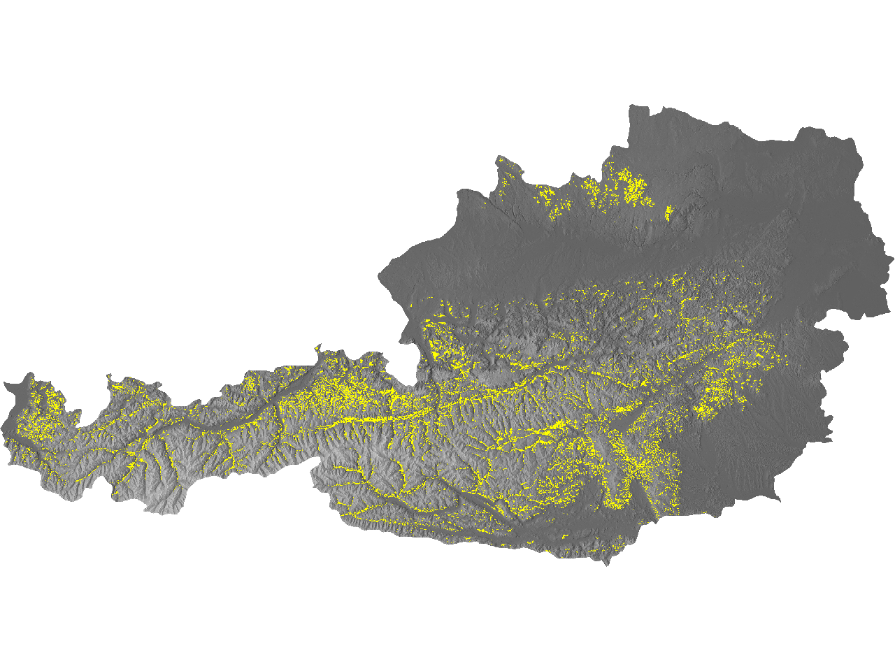
 Shaded EU-DEM with potential range of habitat 6520 (yellow):

Shaded EU-DEM with potential range of habitat 6520 (yellow) and footslopes (search window =3; red) by r.geomorphon:

Shaded EU-DEM with potential range of habitat 6520 (yellow) and footslopes (search window =6; blue) by r.geomorphon:

More investigations are needed. But r.geomorphon is an interesting GIS tool for calculating/defining landforms and landform elements.

Mountain hay meadows - a case for EU-DEM and Corine landcover?

Mountain hay meadows are of European community interest as listed as habitat 6520 in the Habitat Directive and characterized as a biodiversity hotspot [1].

These species-rich mesophile hay meadows of the montane and sub-alpine levels (mostly above 600 metres) are usually dominated by Trisetum flavescens and with Heracleum sphondylium, Viola cornuta, Astrantia major, Carum carvi, Crepis mollis, C. pyrenaica, Bistorta major, (Polygonum bistorta), Silene dioica, S. vulgaris, Campanula glomerata, Salvia pratensis, Centaurea nemoralis, Anthoxanthum odoratum, Crocus albiflorus, Geranium phaeum, G. sylvaticum, Narcissus poeticus, Malva moschata, Valeriana repens, Trollius europaeus, Pimpinella major, Muscari botryoides, Lilium bulbiferum, Thlaspi caerulescens, Viola tricolor ssp. subalpina, Phyteuma halleri, P. orbiculare, Primula elatior, Chaerophyllum hirsutum and many others.[2]

Where are these species-rich mesophile hay meadows? Let's try a quick and dirty approach powered by GRASS GIS 7svn and publicly available GIS data.

Recently a EU-DEM was published and ready for public download: [3]

"The Digital Elevation Model over Europe from the GMES RDA project (EU-DEM) is a Digital Surface Model (DSM) representing the first surface as illuminated by the sensors. The EU-DEM dataset is a realisation of the Copernicus programme, managed by the European Commission, DG Enterprise and Industry. The EU-DEM is a hybrid product based on SRTM and ASTER GDEM data fused by a weighted averaging approach."

link to EU-DEM

r.external --verbose input=C:\myrast\EUD_CP-DEMS_4500025000-AA\EUD_CP-DEMS_4500025000-AA\EUD_CP-DEMS_4500025000-AA.tif output=eudem

crop the EU-DEM to the extent of Austria by Natural Earth country vector data

g.region -p -a rast=eudem vect=ne_10m_admin_0_countries_at_epsg3035 align=eudem
r.mask --verbose vector=ne_10m_admin_0_countries_at_epsg3035
r.mapcalc expression=eudem_austria = eudem@trisetum

 

Corine landcover data is able to spatially indicate to pastures and grassland. Let's try: 231 - Pastures, 243 - Land principally occupied by agriculture, with significant areas of natural vegetation, 321 - Natural grasslands. [5]

import Corine land cover 2006 seamless vector data restricted to Austria's bounding box

v.in.ogr dsn=C:\myvect\corine2012\clc-2006-vector-data-version-2\clc06_c231.1\clc06_c231.shp spatial=4284730,2595723,4853722,2889837
v.in.ogr dsn=C:\myvect\corine2012\clc-2006-vector-data-version-2\clc06_c243.1\clc06_c243.shp spatial=4284730,2595723,4853722,2889837
v.in.ogr dsn=C:\myvect\corine2012\clc-2006-vector-data-version-2\clc06_c321.1\clc06_c321.shp spatial=4284730,2595723,4853722,2889837

select spatially Corine landcover data for Austria's extent

v.select ainput=clc06_c231 binput=ne_10m_admin_0_countries_at_epsg3035 output=clc06_c231_at operator=within
v.select ainput=clc06_c243 binput=ne_10m_admin_0_countries_at_epsg3035 output=clc06_c243_at operator=within
v.select ainput=clc06_c321 binput=ne_10m_admin_0_countries_at_epsg3035 output=clc06_c321_at operator=within

add and update numerical column for a later rasterization

v.db.addcolumn map=clc06_c321_at columns=cdis integer  
v.db.addcolumn map=clc06_c243_at columns=cdis integer
v.db.addcolumn map=clc06_c231_at columns=cdis integer
v.db.update map=clc06_c321_at layer=1 column=cdis value=1
v.db.update map=clc06_c243_at layer=1 column=cdis value=1 
v.db.update map=clc06_c231_at layer=1 column=cdis value=1

rasterize Corine landcover data for later masked raster calculations

v.to.rast input=clc06_c231_at type=area output=rast_clc06_c231_at use=attr attrcolumn=cdis
v.to.rast input=clc06_c243_at type=area output=rast_clc06_c243_at use=attr attrcolumn=cdis
v.to.rast input=clc06_c321_at type=area output=rast_clc06_c321_at use=attr attrcolumn=cdis

patch rasterized Corine landcover data

r.patch input=rast_clc06_c231_at,rast_clc06_c243_at,rast_clc06_c321_at output=corine_pastures_grassland

In literature [2] [6] the altitudinal range of mountain hay meadows is given as 600-800m up to 1.400-1.700m. Let's assume 700 - 1.700m here in these calculations.

calculate altitude range 700 - 1.700m of the EU-DEM
 
r.mapcalc expression=eu_dem_haymeadows_range = if( eudem_austria >= 700 && eudem_austria <= 1700 , 1 )

By combining Corine landcover of pastures and grassland and altitude range we may get some impression of the habitat's potential range.

combine altitude range and corine information

r.mapcalc expression=eu_dem_haymeadows_range_corine = if( eu_dem_haymeadows_range == 1 && corine_pastures_grassland == 1 , 1  , null()  )

As we know that pastures and meadows in more ore less flat areas are intensively and heavily used nowadays, species-rich mesophile habitats are getting infrequent. So let's bring slope into calculations.

calculate slope

r.slope.aspect --verbose elevation=eudem_austria slope=eudem_austria_slope_degree

Therefore let's cut very flat, but also very steep areas where other habitats are getting more dominant. So let's refine potential areas by cutting < 3° and > 22°.

slope raster masked by the Corine landcover-altitudinal-range raster and cut steep areas

r.mapcalc expression=eudem_austria_slope_degree_masked_refined = if( eudem_austria_slope_degree_masked >= 3 && eudem_austria_slope_degree_masked <= 22 , 1 , null() )

Let's zoom in parts of Tyrol without considering slope

and with slope taken into account for refinement.

It is a nice example that two GIS datasets available to the public and open source GIS software allow a very rough estimation of a habitat's potential range by a quick and dirty approach. Although ground proving and more parameters (e.g. geology, shading, exposition, usage, etc.) are really needed for refinement.

Let's start with ground proving in summer time ... :-)

[1] Initiative Rettet die Blumenwiesen
[2] Interpretation Manual of European Union Habitats (EUR 28, April 2013)
[3] EU-DEM
[4] Natural Earth data - Admin 0 – Countries
[5] Corine Land Cover 2006 seamless vector data 
[6] UBA 2005. Entwicklung von Kriterien, Indikatoren und Schwellenwerten zur Beurteilung des Erhaltungszustandes der Natura 2000-Schutzgüter.