Alpine gravel-bed rivers ... seen from far above in the orbit

River ecosystems are connected on large spatial scales, have varied drivers, strong, and often conflicting, societal interests, and interacting management processes. Rivers and riverine landscapes are ecosystems significantly shaped by recurrent natural disturbances. These dynamic processes initiate a complex mosaic of  habitats resulting in a remarkable high diversity of aquatic, amphibious and terrestrial organisms linked

Alpine gravel-bed rivers are of European interest due to 2 directives: Habitats Directive and Water Framework Directive. Regarding Habitats Directive three typical habitats are listed and can be seen as a succession from highly dynamic (3220 Alpine rivers and the herbaceous vegetation along their banks) to medium dynamic (3230 Alpine rivers and their ligneous vegetation with Myricaria germanica) and moderately dynamic (3240 Alpine rivers and their ligneous vegetation with Salix elaeagnos) pioneer sites.

Let's have a look from the orbit at one of the last near natural alpine gravel-bed rivers in the Eastern Alps: Tagliamento.

View to North from Monte Ragogna over Tagliamento's riverine landscape (photo: H. Kudrnovsky)

Ingedients:

• Landsat 8 data
• GRASS GIS
• GDAL

Landsat 8 Operational Land Imager (OLI) and Thermal Infrared Sensor (TIRS) images consist of nine spectral bands with a spatial resolution of 30 meters for Bands 1 to 7 and 9. New band 1 (ultra-blue) is useful for coastal and aerosol studies. New band 9 is useful for cirrus cloud detection. The resolution for Band 8 (panchromatic) is 15 meters. Thermal bands 10 and 11 are useful in providing more accurate surface temperatures and are collected at 100 meters. Approximate scene size is 170 km north-south by 183 km east-west.

Landsat 8 data is available for download at no charge (e.g. Earth Explorer) and with no user restrictions.

First download Landsat 8 data and do a data check by gdalinfo:

Driver: GTiff/GeoTIFF
Files: LC81920282015221LGN00_B1.TIF
Size is 7651, 7771
Coordinate System is:
PROJCS["WGS 84 / UTM zone 32N",
    GEOGCS["WGS 84",
        DATUM["WGS_1984",
            SPHEROID["WGS 84",6378137,298.257223563,
                AUTHORITY["EPSG","7030"]],
            AUTHORITY["EPSG","6326"]],
        PRIMEM["Greenwich",0],
        UNIT["degree",0.0174532925199433],
        AUTHORITY["EPSG","4326"]],
    PROJECTION["Transverse_Mercator"],
    PARAMETER["latitude_of_origin",0],
    PARAMETER["central_meridian",9],
    PARAMETER["scale_factor",0.9996],
    PARAMETER["false_easting",500000],
    PARAMETER["false_northing",0],
    UNIT["metre",1,
        AUTHORITY["EPSG","9001"]],
    AUTHORITY["EPSG","32632"]]

Landsat 8 data is organized in UTM zones; here along the catchment of river Tagliamento UTM zone 32N. Import or link the data into a GRASS location created with EPSG: 32632 (UTM zone 32N).

Band 8 – Panchromatic (resolution 15m x 15m)

Let's have a look at the Landsat data within GRASS GIS:

i.landsat.toar -p input=LC81920282015221LGN00_B output=landsat_toar metfile=LC81920282015221LGN00_MTL.txt lsatmet=number,creation,date,sun_elev,sensor,bands,sunaz,time
number=8
creation=2015-08-09
date=2015-08-09
sun_elev=55.616710
sensor=OLI/TIRS
bands=11
sunaz=144.774232

The -p flag of the i.landsat.toar tool prints metadata info like sun azimuth, sun zenit (=elevation) and others.

Further i.landsat.toar is used to transform the calibrated digital number of Landsat imagery products to top-of-atmosphere radiance or top-of-atmosphere reflectance and temperature. Optionally, it can be used to calculate the at-surface radiance or reflectance with atmospheric correction (DOS method).  Atmospheric correction could also be done later by the dedicated i.atcorr tool.

Let's do the transformation with an atmospheric correction:

i.landsat.toar --verbose input=LC81920282015221LGN00_B output=dos1_corr_toar metfile=LC81920282015221LGN00_MTL.txt sensor=oli8 method=dos1

By i.colors.enhance an auto-balancing of colors for RGB images is performed.

i.colors.enhance red=dos1_corr_toar4 green=dos1_corr_toar3 blue=dos1_corr_toar2

RGB image (resolution 30m x 30m)

Habitat 3220 Alpine rivers and the herbaceous vegetation along their banks is typical for slightly vegetated gravel banks. Such sites often shows a high albedo. i.albedo computes broad band albedo from surface reflectance. In order to speed up computation time, e.g. the river (e.g. extracted from Natural Earth) can be buffered and a mask set by this buffer.

i.albedo -l -c --verbose input=dos1_corr_toar2,dos1_corr_toar3,dos1_corr_toar4,dos1_corr_toar5,dos1_corr_toar6,dos1_corr_toar7 output=tag_albedo_aggressivemode

i.albedo result; albedo raster values above a manually chosen threshold (here e.g. 0.19) clumped and vectorized

vectorized albedo above threshold 0.19 overlayed over a RGB image

The normalized difference vegetation index (NDVI) is a simple graphical indicator that can be used to analyze remote sensing measurements and assess whether the target being observed contains live green vegetation or not.

i.vi red=dos1_corr_toar4 output=vi_nvdi viname=nvdi nir=dos1_corr_toar5 green=dos1_corr_toar3 blue=dos1_corr_toar2 band5=dos1_corr_toar6t band7=dos1_corr_toar7

vectorized albedo above threshold 0.19 overlayed over a  NDVI map

vectorized albedo above threshold 0.19 overlayed over a panchromatic Landsat 8 image

linking albedo analysis with nature

As the Landsat 8 satellite images the entire Earth every 16 days in an 8-day offset from Landsat 7, temporal and spatial analysis of alpine rivers and their gravel bed riverine landscape may be viable over large scale.

Combining available open source software (e.g. GRASS GIS, QGIS, Orfeo ToolBox) with open data (e.g. Landsat, Sentinel) tweaked by ground proofing may support to fulfill the targets of the EU directives (Habitats Directive, Water Framework Directive): sustainable water use and biodiversity preservation.

Forests of temperate Europe in the light of open data, open source software and SQL

According to the interpretation manual of the EU habitat directive some forests of community interest in the region of the temperate Europe are:

• 9110 Luzulo-Fagetum beech forests 
• 9120 Atlantic acidophilous beech forests with Ilex and sometimes also Taxus in the shrublayer (Quercinion robori-petraeae or Ilici-Fagenion)
• 9130 Asperulo-Fagetum beech forests
• 9140 Medio-European subalpine beech woods with Acer and Rumex arifolius
• 9150 Medio-European limestone beech forests of the Cephalanthero-Fagion
• 9160 Sub-Atlantic and medio-European oak or oakhornbeam forests of the Carpinion betuli
• 9170 Galio-Carpinetum oak-hornbeam forests
• 9180 * Tilio-Acerion forests of slopes, screes and ravines
• 9190 Old acidophilous oak woods with Quercus robur on sandy plains

Some open ingredients for baking an analysis around these forests:

• Natura 2000 data - the European network of protected sites
• Natural Earth Admin 0 – Countries
• SQLite - an open software library that implements a self-contained, serverless, zero-configuration, transactional SQL database engine
• SpatiaLite - open source library to extend the SQLite core to support fully fledged Spatial SQL capabilities
• GDAL/OGR
• QGIS

First download the spatialite version of the Natura 2000 data and have a quick look into the database by ogrinfo:

ogrinfo Natura2000_end2014.sqlite
INFO: Open of `Natura2000_end2014.sqlite'
      using driver `SQLite' successful.
1: natura2000polygon (Multi Polygon)

Beside the spatial data of protected areas within the Natura 2000 network (multipolygon layer: natura2000polygon), the database version of this data inlcudes also already additional informations connected to the protected areas (bioregion, contacts, designation status, directive species, habitat classes, habitats, impact, management, meta data, natura 2000 sites, other species, species).

Let's have a deeper look into the spatialite database (simplified by e.g. the spatialite-gui) and do some non-spatial SQL queries; e.g. filtering/querying the data and creating a view of protected areas including 9110 Luzulo-Fagetum beech forests:

# create view with protected areas including 9110 Luzulo-Fagetum beech forests based on the non-spatial table HABITATS
CREATE VIEW "vhabitat9110" AS
SELECT "SITECODE" AS "SITECODE", "HABITATCODE" AS "HABITATCODE",
    "COVER_HA" AS "COVER_HA", "REPRESENTATIVITY" AS "REPRESENTATIVITY",
    "RELSURFACE" AS "RELSURFACE", "CONSERVATION" AS "CONSERVATION",
    "GLOBAL_ASSESMENT" AS "GLOBAL_ASSESMENT", "DATAQUALITY" AS "DATAQUALITY",
    "PERCENTAGE_COVER" AS "PERCENTAGE_COVER"
FROM "HABITATS"
WHERE "HABITATCODE" = 9110
ORDER BY "SITECODE";

A view is some kind of a filtered/queried view of data organized like a table.

Just do it analogously for the other forest habitat types.

Then implement a spatial view of the data for later loading it to GIS:

# join the view created in the step before (vhabitat9110) with the spatial layer (Natura2000polygon) of the spatialite database.
CREATE VIEW "svhabitat9110" AS
SELECT "a"."ROWID" AS "ROWID", "a"."PK_UID" AS "PK_UID",
    "a"."SITECODE" AS "SITECODE", "a"."SITENAME" AS "SITENAME",
    "a"."RELEASE_DA" AS "RELEASE_DA", "a"."MS" AS "MS",
    "a"."SITETYPE" AS "SITETYPE", "a"."Geometry" AS "Geometry",
    "b"."SITECODE" AS "SITECODE_1", "b"."HABITATCODE" AS "HABITATCODE",
    "b"."COVER_HA" AS "COVER_HA", "b"."REPRESENTATIVITY" AS "REPRESENTATIVITY",
    "b"."RELSURFACE" AS "RELSURFACE", "b"."CONSERVATION" AS "CONSERVATION",
    "b"."GLOBAL_ASSESMENT" AS "GLOBAL_ASSESMENT", "b"."DATAQUALITY" AS "DATAQUALITY",
    "b"."PERCENTAGE_COVER" AS "PERCENTAGE_COVER"
FROM "Natura2000polygon" AS "a"
JOIN "vhabitat9110" AS "b" USING ("SITECODE")
ORDER BY "a"."SITECODE";

# registration of the spatial view to be loadable for GIS
INSERT INTO views_geometry_columns
    (view_name, view_geometry, view_rowid, f_table_name, f_geometry_column, read_only)
  VALUES ('svhabitat9110', 'geometry', 'rowid', 'natura2000polygon', 'geometry', 1);

A spatial view is some kind of a filtered/queried view of spatial data organized in a spatial database.

Do the same also for the other forest habitat types and have a look into the database:

ogrinfo Natura2000_end2014.sqlite
INFO: Open of `Natura2000_end2014.sqlite'
      using driver `SQLite' successful.
1: natura2000polygon (Multi Polygon)
2: svhabitat9110 (Multi Polygon)
3: svhabitat9120 (Multi Polygon)
4: svhabitat9130 (Multi Polygon)
5: svhabitat9140 (Multi Polygon)
6: svhabitat9150 (Multi Polygon)
7: svhabitat9160 (Multi Polygon)
8: svhabitat9170 (Multi Polygon)
9: svhabitat9180 (Multi Polygon)
10: svhabitat9190 (Multi Polygon)

Now there are spatial views of several forest habitat types.

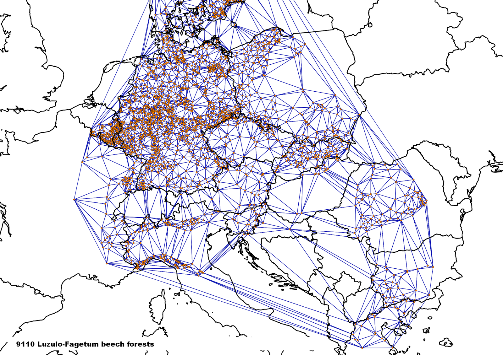
Open QGIS, load the spatial views of protected areas with forest and let's do some further analysis, e.g. calculate the polygon centroids (in QGIS: Vector -> Geometry tools -> Polygon centroid) and a Delaunay triangulation of the centroids (in QGIS: Vector -> Geometry tools -> Delaunay triangulation) showing the function of an ecological network of protected areas for a certain habitat type in a simple way.

Some overviews of the distribution of some European temperate forest types within the Natura 2000 network by centroids of protected areas, connected by a Delaunay triangulation:

9110 Luzulo-Fagetum beech forests

9120 Atlantic acidophilous beech forests with Ilex and sometimes also Taxus in the shrublayer (Quercinion robori-petraeae or Ilici-Fagenion)

9130 Asperulo-Fagetum beech forests

9140 Medio-European subalpine beech woods with Acer and Rumex arifolius

9150 Medio-European limestone beech forests of the Cephalanthero-Fagion

9160 Sub-Atlantic and medio-European oak or oakhornbeam forests of the Carpinion betuli

9170 Galio-Carpinetum oak-hornbeam forests

9180 * Tilio-Acerion forests of slopes, screes and ravines

9190 Old acidophilous oak woods with Quercus robur on sandy plains

Another nice example of a interaction/interplay of open data and open source software to get an overview of European nature.

Joint effort needed for biodiversity

Open data and open source software may be a guide for such an joint effort. Let's have a look on the data side at ressources of EEA, GBIF and Natural Earth, on the software side at QGIS and R.

GBIF facilitates free and open access to biodiversity data, e.g. species distribution data. This kind of data can be accessed and processed by R and its packages dismo, sp, rgdal and maptools.

# load libraries
library(sp)
library(dismo)
library(rgdal)
library(maptools)

# download species distribution data as spatial points data frame, e.g. Myricaria germanica
myrger <- gbif("Myricaria", "germanica", geo = TRUE, sp = TRUE, removeZeros = TRUE)

# visualize data for a quick check
data(wrld_simpl)
plot(wrld_simpl, col = "light yellow", axes = T)
points(myrger$lon, myrger$lat, col = "red", cex = 0.5)
text(-140, -50, "Myricaria\ngermanica")

GBIF species distribution data of Myricaria germanica (accessed: 2014-11-18)

# define projection of the spatial data
proj4string(myrger) <- "+proj=longlat +datum=WGS84"

# export to shape file to use it in QGIS
writeOGR(myrger3, dsn = ".", driver= "ESRI Shapefile", layer = "gbif_mg_ll")

Natural Earth has a nice compilation of cultural, physical and raster GIS data; in this example the boundaries of countries are used. The European Environment Agency (EEA) delivers data of the biogeographical regions and the article 17 report GIS data on the conservation status of habitat types and species for the reporting period 2001-2006 required by the Habitat directive. The European Topic Centre on Biological Diversity supplies data of the article 17 report for the period 2007-2012.

Let's collect all the GIS data for e.g. habitat type "3230 Alpine rivers and their ligneous vegetation with Myricaria germanica" and load the data into QGIS. Data for France and Slovenia of the reporting period 2007-2012 isn't available yet.

Data: countries - Natural Earth; biogeographical regions and article 17 period 2001-2006 - EEA;
article 17 period 2007-2012 - European Topic Centre on Biodiversity

And zoom into several European mountain regions:

Pyrenees

Carpathians

Scandinavian mountains

Scandinavian mountains quite in the North

Alps

A closer look to Austria

Austria

and a recent article about the actual and historic distribution of Myricaria germanica in Austria (Stapfia 99; see also here)

taken from Kudrnovsky & Stöhr, 2013. Myricaria germanica (L.) Desv. historisch und aktuell in Österreich: ein dramatischer Rückgang einer Indikatorart von europäischem Interesse. STAPFIA 99 (2013): 13–34.

As differences in the state of knowledge and differences in important datasets like GBIF and article 17 report are getting obvious, a joint effort of knowlegde transfer and boosted data exchange may be needed to achieve the targets of the EU Biodiversity Strategy to 2020.